documentation
The Rosetta mission
The International ROSETTA Mission was the planetary cornerstone mission in ESA's long-term programme “Horizon 2000” approved in November 1993. It was a cooperative project between ESA, several European national space agencies, and NASA. Its main scientific objective was to investigate the origin of our solar system by performing in-situ observations of a comet, a member of a family of objects thought to be the most primitive. The mission was conceived as a rendezvous with its target comet while inactive at a large heliocentric distance so as to allow studying its nucleus, followed by an escort phase to and past perihelion to characterize the development of cometary activity. Trajectory analysis indicated that it was possible to fly by up to two asteroids during the journey to the comet. Final selection, once the launch date was firmly established, led to choosing comet 67P/Churyumov–Gerasimenko as the main target of the rendezvous and asteroids (2867) Steins and (21) Lutetia as flyby targets (Fig. 1). The spacecraft consisted of two mission elements, the ROSETTA orbiter and the ROSETTA lander PHILAE altogether comprising a suite of 21 scientific instruments (Glassmeier et al. 2007).
After its launch on 2 March 2004 with an Ariane V rocket, the spacecraft started its long journey to the comet. Four gravity assists, three by Earth and one by Mars were required to propel the ROSETTA spacecraft to a distance of 3.6 AU to rendezvous with the comet. During this cruise phase, ROSETTA flew by asteroids (2867) Steins on 5 September 2008 and (21) Lutetia on 10 July 2010, see Fig. 1 and the animation in the following movie.
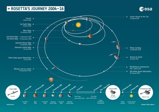
Fig. 1: The interplanetary trajectory of the ROSETTA spacecraft
The spacecraft was put in a state of deep space hibernation during 31 months and woken up on 20 January 2014. It arrived at a distance of 100 km from the nucleus on 6 August 2014 and then started a complex journey around the nucleus in order to fulfill its scientific mission as illustrated in the following ESA animation:
Various constraints besides scientific dictated this circum-cometary navigation, particularly the safety of the spacecraft. Consequently, its distance to the nucleus varied considerably as illustrated in Fig. 2 and conspicuously increased around perihelion time as a measure of protection against the increasing cometary activity.
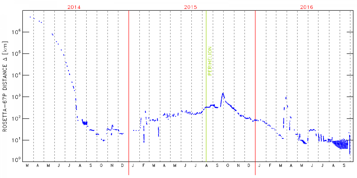
Fig. 2: Evolution of the distance (in km) between the ROSETTA spacecraft and the nucleus of comet 67P/Churyumov–Gerasimenko from March 2014 to September 2016 using a logarithmic scale. The blue dots corresponds to images taken by the OSIRIS Narrow Angle Camera (NAC, see next section) for a total amount of 26827 images.
The OSIRIS-NAC instrument
OSIRIS, the Optical, Spectroscopic, and Infrared Remote Imaging System of the ROSETTA mission (OSIRIS) consisted of a Narrow Angle Camera (NAC) and a Wide Angle Camera (WAC) operating in the visible, near infrared and near ultraviolet wavelength ranges (Keller et al. 2007). OSIRIS was built by a consortium of the Max-Planck-Institut für Sonnensystemforschung, Göttingen, Germany, CISAS-University of Padova, Italy, the Laboratoire d’Astrophysique de Marseille, France, the Instituto de Astrofísica de Andalucía, CSIC, Granada, Spain, the Scientific Support Office of the European Space Agency, Noordwijk, Netherlands, the Instituto Nacional de Técnica Aeroespacial, Madrid, Spain, the Universidad Politéchnica de Madrid, Spain, the Department of Physics and Astronomy of Uppsala University, Sweden, and the Institut für Datentechnik und Kommunikationsnetze der Technischen Universität Braunschweig, Germany.
All anaglyphs presented on this website were constructed from images taken by the OSIRIS-NAC (Lamy et al. 2019). Its telescope was conceived and developed by the Laboratoire d’Astrophysique de Marseille in partnership with ASTRIUM (Toulouse) and with the European institutes of the consortium. Its optical concept implemented the three-mirror anastigmat (TMA) solution (Fig. 3) insuring low stray light by eliminating the central obscuration present in axial designs. The optimized solution required only two aspheric mirrors, the tertiary remaining spherical. It ensured a flat field, an axial pupil and an off-axis field of view of 2.20°x2.22°. The telescope was equipped with a 2048 × 2048 pixel backside illuminated CCD detector with a UV optimized anti-reflection coating. The pixel size of 13.5 µm yielded an image scale of 3.9 arcsec/pixel. The NAC was equipped with 11 filters mounted on two filter wheels and covering a wavelength range of 250 to 1000 nm (Fig. 4).
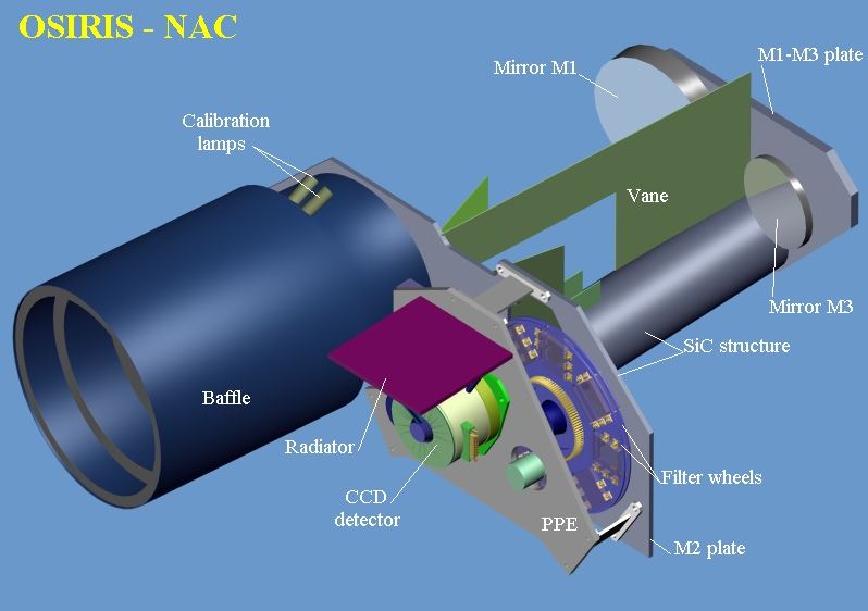
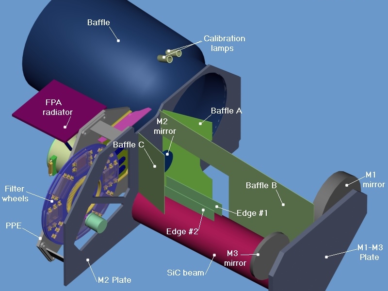
Fig. 3: Two schematic views of the OSIRIS Narrow Angle Camera.
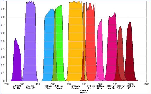
Fig. 4: The spectral transmission curves of the 11 filters of the OSIRIS-NAC.
The images used to build the anaglyphs were obtained with 13 filters:
F16, F22, F23, F24, F27, F28, F41, F51, F61, F71, F82, F84, F88. Their properties are given in the following Table:
| Code | Name | λc | Δλ | |
| _______________________________________ | ||||
| F16 | Near UV | 367.6 | 36.7 | |
| F22 | Orange | 648.6 | 85.2 | |
| F23 | Green | 536.4 | 64.5 | |
| F24 | Blue | 479.9 | 74.0 | |
| F27 | Hydra | 701.2 | 22.0 | |
| F28 | Red | 742.4 | 63.2 | |
| F41 | Near IR | 880.1 | 63.6 | |
| F51 | Ortho | 804.7 | 40.6 | |
| F61 | Fe2O3 | 931.7 | 34.7 | |
| F71 | IR | 986.1 | 34.5 | |
| F82 | F22 + Neutral density filter | |||
| F84 | F24 + Neutral density filter | |||
| F88 | F28 + Neutral density filter | |||
| ________________________________________ | ||||
λc = central wavelength, Δλ = bandwith (nm)
A view of the flight model of the NAC (without its thermal blanket) during final testing at Laboratoire d’Astropysique de Marseille is shown in Fig. 5.
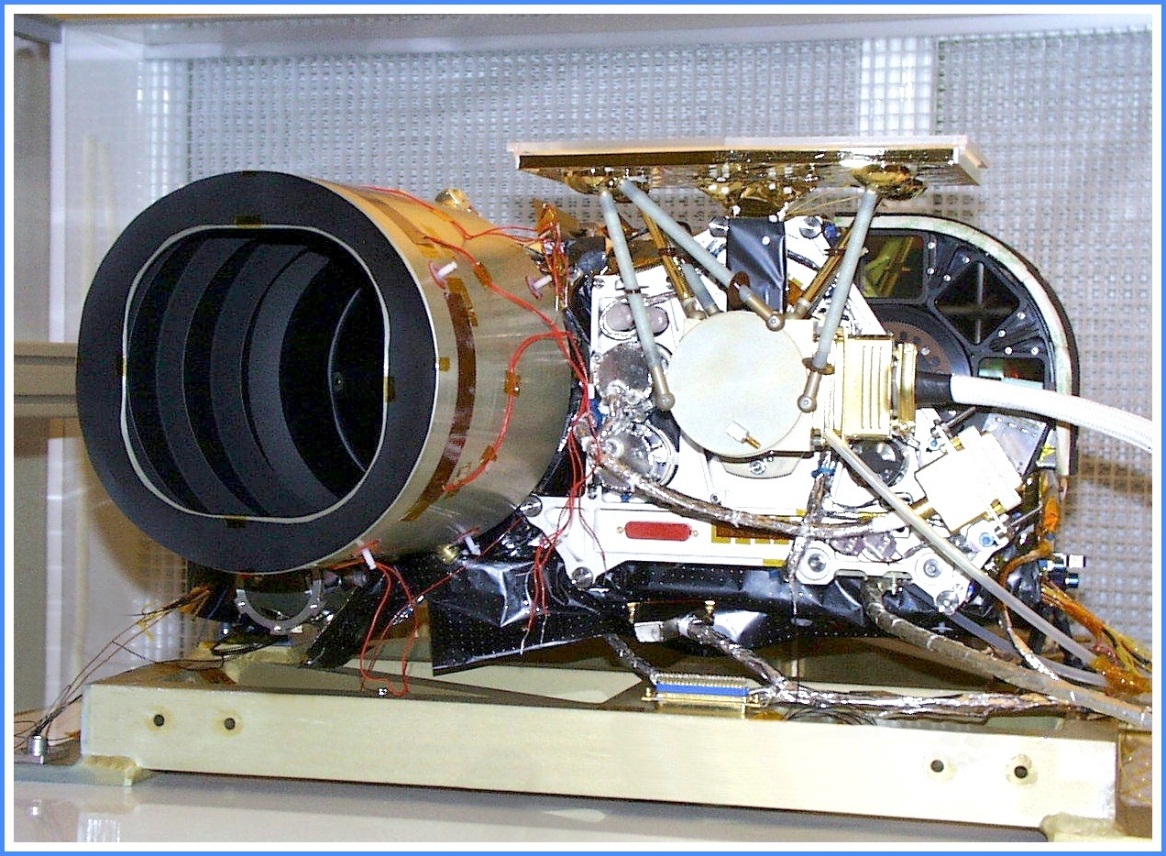
Fig. 5: The flight model of OSIRIS-NAC.
The processing of the OSIRIS images
All OSIRIS images went through a complex, two-step calibration pipeline. The first step converted the raw data downloaded from the spacecraft to level-1 images with calibrated hardware parameters and S/C pointing information. The second step converted these level-1 images to radiometric calibrated and geometric distortion corrected images (level 2 and 3, respectively) through a series of successive tasks as illustrated in the flowchart of Fig. 6 (Tubiana et al. 2015). An additional level-4 was later implemented to associate to each pixel of each image its cometo-centric coordinates (longitude and latitude) so as to precisely localize the images on the nucleus.
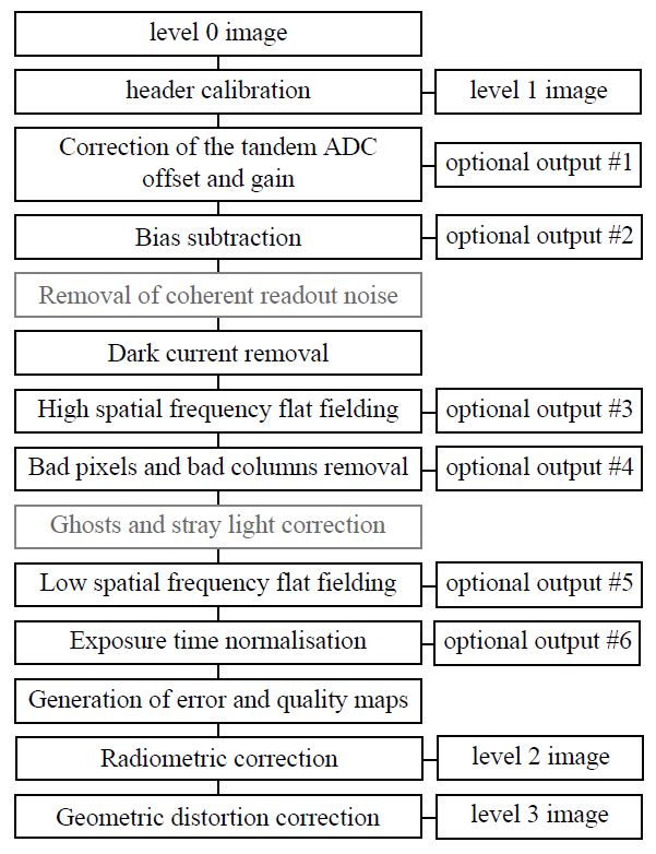
Fig. 6: Flowchart of the OSIRIS calibration pipeline (reproduced from Fig. 2 of Tubiana et al., 2015).
The construction of the stereo anaglyphs
The potential of direct stereoscopic views of the nucleus of comet 67P/Churyumov–Gerasimenko was never realized during the preparation of the observational program of the NAC. The emphasis was put on the construction of numerical 3D models and digital terrain models (DTMs) since they provide quantitative information. Fortunately, it turned out that many observational programs required sequences of concatenated images so that a large number of image pairs were subsequently found suitable for anaglyph construction once it was realized that they offered fantastic views of the nucleus and could be helpful in understanding the relief of its surface. Optimal conditions for stereo imaging require two identical cameras spaced for stereo base and taking images at the same time to insure identical illumination conditions. Evidently, these optimal conditions were not met by the OSIRIS camera system. With only one high resolution camera, the NAC, the stereo effect had to rely on its displacement. In practice, two effects came into play: the motion of the spacecraft and the intrinsic rotation of the nucleus, they relative importance depending upon the distance between the camera and the nucleus. The displacement is not arbitrary and must reproduce human vision with a stereoscopic base of 7 cm, the typical distance between our two eyes. This distance is adequate to introduce projection differences, so-called parallax, between 30 cm and several hundred meters. A horizontal parallax commonly considered as comfortable for the brain is ≈2° corresponding to a base of ≈1/30 of the distance to the near object, values which are adapted to the focal length of our eyes. After pre-selecting pairs of images on the basis of their time interval, the parallax between the two images is estimated and serves as a criterion for the final selection. In practice, the criterion was relaxed to a range of parallax adapted to different conditions of visualization of the resulting anaglyphs. A parallax of ≈2° is appropriate to viewing the anaglyph on a computer screen. A parallax of ≈0.5°, that is a base of 1/100, is suitable to a projection on a large screen at a conference. A parallax of ≈3.8°, that is a base of 1/15, is adapted to smartphones. A few anaglyphs with a parallax larger than 4° (base < 1/10), a limit beyond which the depth becomes too dilated, have been kept when presenting a specific interest. As it will be explained in the next session, the value of the base is included in the name of the anaglyph and the parallax is given as a parameter in the database.
It has been pointed out above that part of the displacement results from the rotation of the nucleus. This has an adverse effect of modifying the cast shadows between the two images thus producing an uncomfortable incoherence perceived as a “vibration” between the limits of the two shadows. This effect can be removed by darkening regions so as to cover the maximum extent of the shadows recorded on both images. We have done so manually on a limited number of anaglyphs of particular value. A systematic correction would be enormously time-consuming and would in fact require the development of an automatic procedure, a task beyond the scope of the present catalog.
Once a pair of suitable images has been selected, the construction of the anaglyph proceeds in several steps.
- A thresholding is applied to both images to adapt them to a common range of brightness (same minima and maxima). This operation is performed with the FITS Liberator software.
- The images are rotated using an image editor software so that their relative displacement is horizontal.
- The anaglyph is then created using the StereoPhoto Maker software of Masuji Suto.
- The anaglyph is finalized using Photoshop or GIMP to perform cosmetics correction, cutting out non-overlapping sections and applying sharpening filters as appropriate. Incoherent shadow limits may also be corrected as explained above.
The earliest anaglyph was constructed from images obtained on 3 August 2014. The subsequent temporal distribution is illustrated in Fig. 7. At time of writing, some 1400 anaglyphs have been produced after considering a subset of nearly 8000 NAC images. It is estimated that a total of 3500 to 4000 anaglyphs could be produced once the whole set of NAC images had been scrutinized.
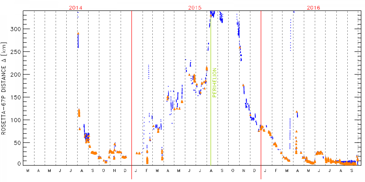
Fig. 7: Same as Fig. 2 except that i) the distance scale is linear and limited to 350 km and ii) the constructed anaglyphs are superimposed as orange triangles.
The parameters of the anaglyphs
Each anaglyph is documented by a set of 17 parameters which provide the contextual information. With the exception of the anaglyphs which show the whole nucleus, the spatial extent of the bulk of them is highly variable depending upon the distance to the comet. A particular attention has been given to their localization on the nucleus. In addition to purely technical information (e.g. coordinates), different levels of localization are presented:
- A global localization in terms of the main components of the nucleus, “big lobe” (BL), “small lobe” (SL), and “neck” (NK). Combinations are of course possible such as BL+NK.
- A regional localization based on the 26 morphological regions defined on the nucleus (El-Maarry et al. 2017)
- A view of one of the image of the anaglyph projected on a 3D model of the nucleus.
An illustration of the 26 regions is presented in Fig. 8 as well as in a movie realized by N. Thomas and co-workers at the Physikalisches Institut, University of Bern. - Click here to see -
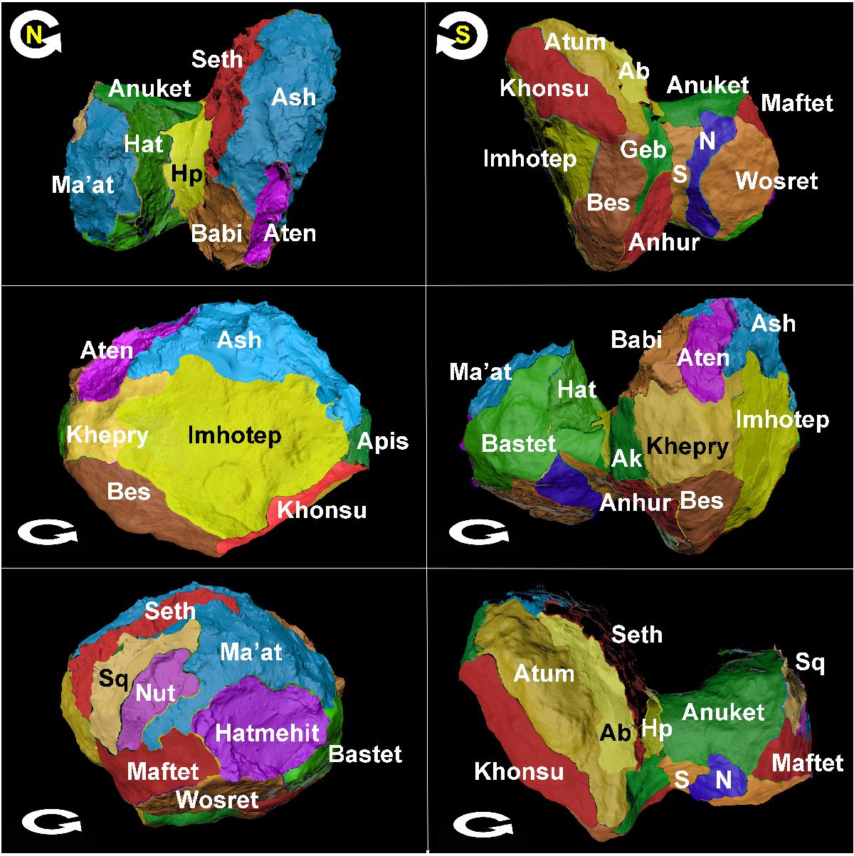
Fig. 8: Six different views of the nucleus of 67P showing the 26 defined regions. The following names have been abbreviated for legibility: Hapi (Hp), Hathor (Hat) Sobek (S), Neith (N), Aker (Ak), and Serqet (Sq). Circular arrows show the direction of the comet’s rotation (reproduced from Fig. 2 of El-Maarry et al. 2017).
For the projection as illustrated in Fig. 9, a global 3D model of the nucleus resulting from a stereo-photogrammetric analysis of more than 1500 NAC images of the nucleus of 67P (Preusker et al. 2017) has been used. This model has 4 million facets and has a spatial resolution of 3.4 m.
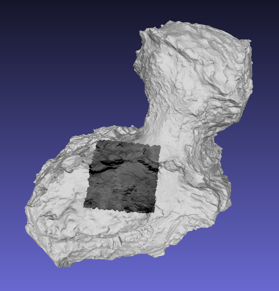
Fig. 9: Illustration of the projection of one of the image of an anaglyph on a 3D model of the nucleus.
The name of an anaglyph concatenates the prefix “anag”, the name of the two images used for its creation, the value expressed by “P1sVAL” (VAL being the inverse of the parallax), and a code for the thresholding (“lin” for linear, “xp1s2” for square root).
The parameters for each anaglyph listed below are part of the database and can therefore be queried in order to select a specific subset of anaglyphs.
• Name of the first image (left/red image)
• Name of the second image (right/cyan)
• Filter of the first image
• Filter of the second image
• Date and time of the earliest image used for the anaglyph
• Global localization of the anaglyph: BL, SL, NK or combination
• Regional composition of the anaglyph
• Longitude of the center of the anaglyph (deg)
• Latitude of the center of the anaglyph (deg)
• Minimum distance to the closest pixel of the anaglyph (km)
• Maximum distance to the farthest pixel of the anaglyph (km)
• Mean distance obtained by averaging the distances of all pixels (km)
• Mean spatial scale of the anaglyph (cm/pixel)
• Size of the anaglyph as mean length and width of the anaglyph (m)
• Phase (Sun-nucleus-Rosetta) angle (deg)
• Parallax of the anaglyph (deg)
• Feature of interest among the following seven items: Jets, Rings, Pancake, Pits, Agilka (the initial landing site of Philae), Abydos (the final landing site of Philae), and Philae.
How to best view the anaglyphs
The anaglyphs of comet 67P/Churyumov–Gerasimenko implements the standard red/cyan system: the left image is coded in red levels and the right image is code in cyan (green+blue) levels. Fusion of the two images is performed by the brain and the scene is seen in relief in gray levels thanks to the additive synthesis of colors. Careful attention must be given to the combination of the red/cyan glasses and the display screen to avoid crosstalk that is leakages, between the two color channels. This adverse effect limits the ability of the brain to successfully fuse the images perceived by each eye and thus reduces the perceived quality of the 3D relief. A simple, basic test can be performed by looking at the anaglyph with only one eye (blocking the other) and checking that a single image in seen (and not two slightly displaced images). For a more comprehensive analysis, we direct the reader to the article by Woods and Harris (2010) who quantified the crosstalk of a very large number of glasses and displays and to the website of David Romeuf:
The anaglyphs must be viewed in subdue light to fully grasp the weakest contrasts in the 3 image that convey relief detail. White bands that may appear on both sides of the displayed anaglyph if it does not fill the screen must be avoided.
Finally, most anaglyphs are of sufficiently quality for deep zooming thus offering dramatically detailed 3D views of the surface of the nucleus of comet 67P/Churyumov–Gerasimenko.
References
Glassmeier, K., Boehnhardt, H., Koschny, D., et al. 2007, Space Sci. Rev. 128, 1.
Keller, H. U., Barbieri, C., Lamy, P., et al. 2007, Space Sci. Rev., 128, 433.
Lamy, P., Faury, G., Romeuf, D., Groussin, O. 2024, MNRAS 531, 2494.
Preusker, F., Scholten, F., Matz, K.-D, et al. 2017, A&A 607, L1.
Tubiana, C., Kovacs, G., Güttler, C., et al. 2015, A&A, 583, 46.
El-Maarry, M. R.,Thomas, N., Gracia-Berná, A., et al. 2017, A&A 598, C2.
Woods, A. J. , Harris, 2010 in Proceedings of SPIE Stereoscopic Displays and Applications XXI, vol. 7253, pp. 0Q1-0Q12.
http://cmst.curtin.edu.au/wp-content/uploads/sites/4/2016/05/2010-11.pdf